IRNSS-1H / PSLV-C39 reentry prediction
Please, see here for the calculations details.
Simulation date: 2019-03-02
Atmosphere model: NRLMSISE-00, data file: 2019 Mar 02 10:00:02.39
Gravity model: SGG-UGM-1 truncated to degree and order 15
Reentry date: 2019-03-02 19:59 ± 3 hours @ 87% confidence level (2019-03-02 16:59 ÷ 2019-03-02 22:59)
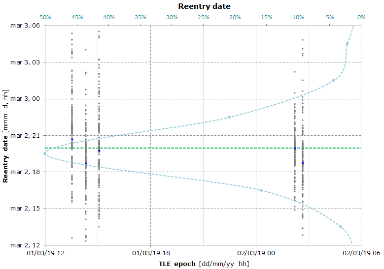
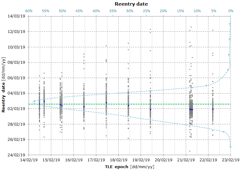
Here's the result of a Monte Carlo simulation used to calculate the reentry date and the reentry location.
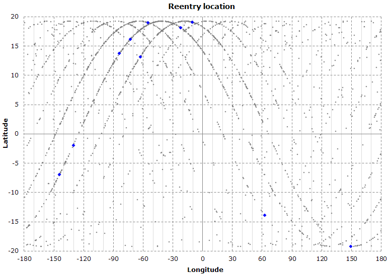
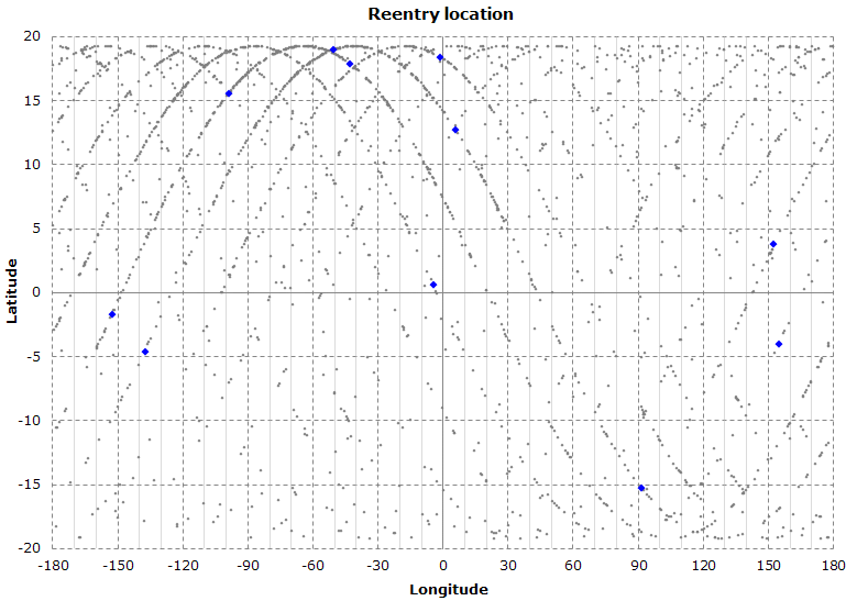
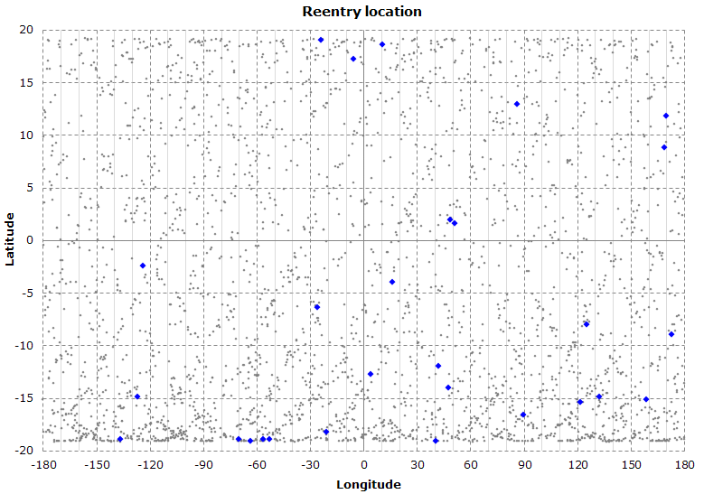
The following map shows the predicted reentry location for each Monte Carlo simulation (the blue dots represent the original, unmodified, TLEs).
If you hover the mouse over a point, a label appears showing the reentry date (TDT) and the TLE epoch.
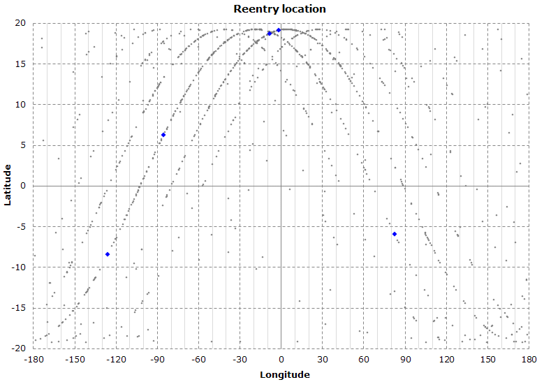
Here's the same as the above map.
The percentage of the reentry locations in the Northern Hemisphere is now 72.8%.
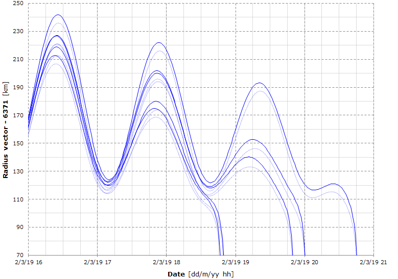
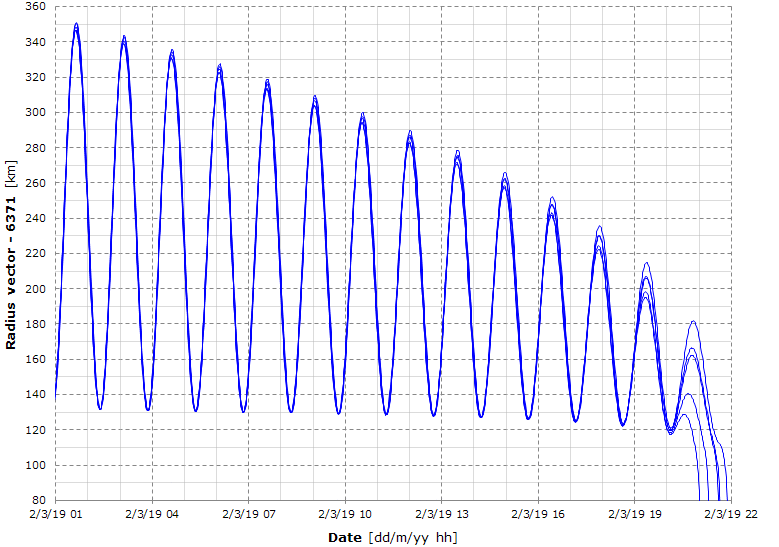
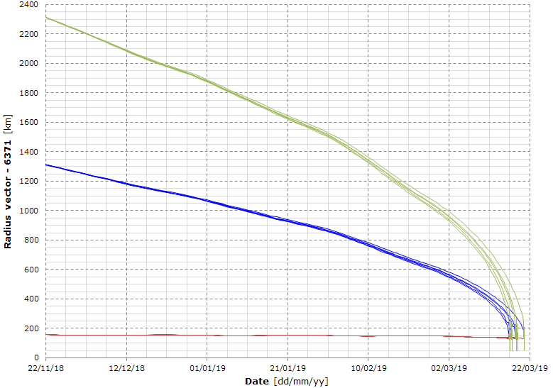
Here's the predicted radius vector propagated from the newest 5 TLEs.
The dotted plots represent the altitude above the WGS-84 ellipsoid.
The following table shows the TLEs used in this simulation and the predicted reentry date:
| TLE epoch |
Reentry date |
| 19060.56388593 | 02/03/2019 20:46 |
| 19060.59658119 | 02/03/2019 18:48 |
| 19060.62765322 | 02/03/2019 19:51 |
| 19061.09218800 | 02/03/2019 20:01 |
| 19061.11119682 | 02/03/2019 18:51 |
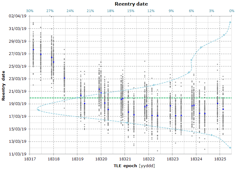
Simulation date: 2019-03-01
Atmosphere model: NRLMSISE-00, data file: 2019 Mar 01 16:00:02.87
Gravity model: SGG-UGM-1 truncated to degree and order 15
Reentry date: 2019-03-02 21:55 ± 21 hours @ 90% confidence level (2019-03-02 00:29 ÷ 2019-03-03 19:22)
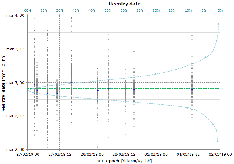
Here's the result of a Monte Carlo simulation used to calculate the reentry date and the reentry location.
The following map shows the predicted reentry location for each Monte Carlo simulation (the blue dots represent the original, unmodified, TLEs).
If you hover the mouse over a point, a label appears showing the reentry date (TDT) and the TLE epoch.
Here's the same as the above map.
The percentage of the reentry locations in the Northern Hemisphere is now 73.9%.
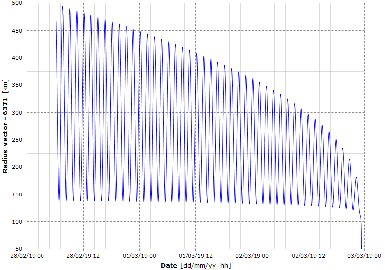
Here's the predicted radius vector propagated from the newest 5 TLEs.
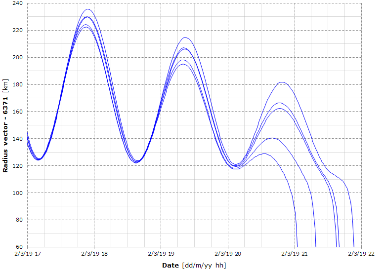
Here's the detailed view of the above graph (notice that this is the radius vector, not the altitude).
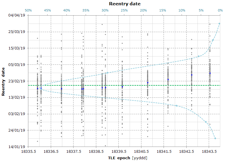
Simulation date: 2019-02-28
Atmosphere model: NRLMSISE-00, data file: 2019 Feb 28 10:00:02.36
Gravity model: SGG-UGM-1 truncated to degree and order 15
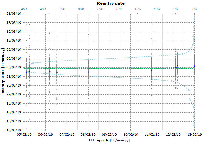
Reentry date: 2019-03-03.0 ± 1.5 days @ 90% confidence level (2019-03-01.5 ÷ 2019-03-04.5)
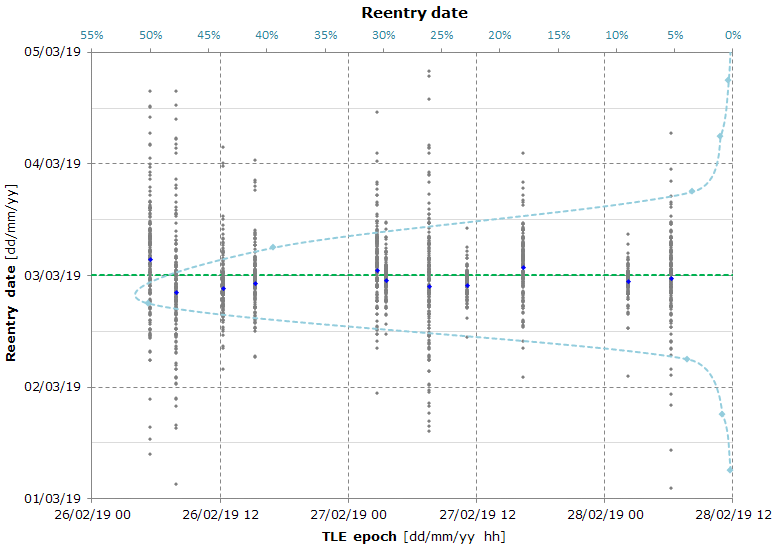
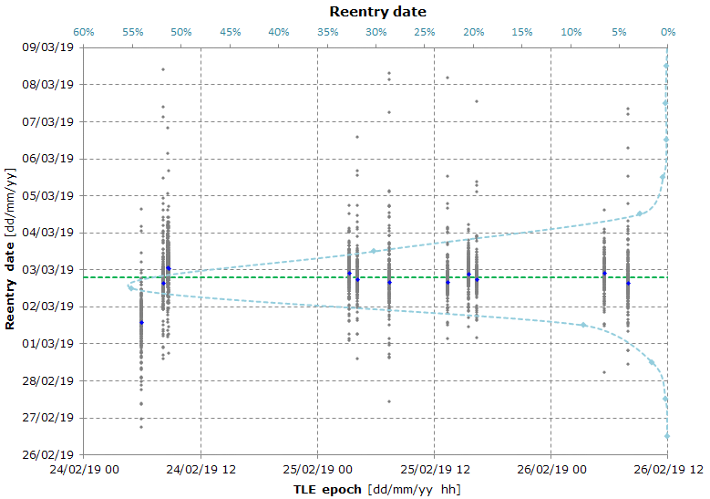
Here's the result of a Monte Carlo simulation used to calculate the reentry date and the reentry location.
| Simulation date |
Reentry date |
| 2019-01-24 | 2019-03-04 07:46 |
| 2019-02-13 | 2019-03-02 15:34 |
| 2019-02-22 | 2019-03-02 13:58 |
| 2019-02-26 | 2019-03-02 19:25 |
| 2019-02-28 | 2019-03-03 00:02 |
Here's the reentry dates obtained from the most recent simulations. We see that, starting from the simulation 2019-02-22, the predicted reentry dates are slightly delayed.
If we take a look at the next table, we can see the reason.
| |
2019-02-22 |
2019-02-26 |
2019-02-28 |
| 2019-02-22 | 170 | 60 | 60 |
| 2019-02-23 | 176 | 30 | 30 |
| 2019-02-24 | 104 | 20 | 20 |
| 2019-02-25 | 104 | 40 | 40 |
| 2019-02-26 | 104 | 118 | 40 |
| 2019-02-27 | 248 | 264 | 160 |
| 2019-02-28 | 280 | 304 | 290 |
| 2019-03-01 | 264 | 248 | 248 |
| 2019-03-02 | 216 | 216 | 216 |
| 2019-03-03 | 176 | 176 | 176 |
Here's the daily sum of the predicted and measured Kp (geomagnetic) index taken from the file
SpaceWeather-All-v1.2.txt (about 2.8 MiB). The bigger the Kp index the bigger the air density.
The table shows the three simulation dates and the predicted/measured daily sum of the Kp index.
We see, for example, that on Feb 22 the predicted daily sum of the Kp index is 170, 176, 104, 104, ..., while the sum of the measured values is 60, 30, 20, 40, ..., the difference is very big and the atmosphere model overestimate the air density and hence the decay rate.
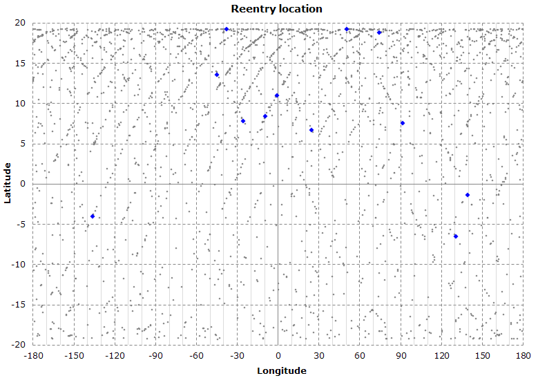
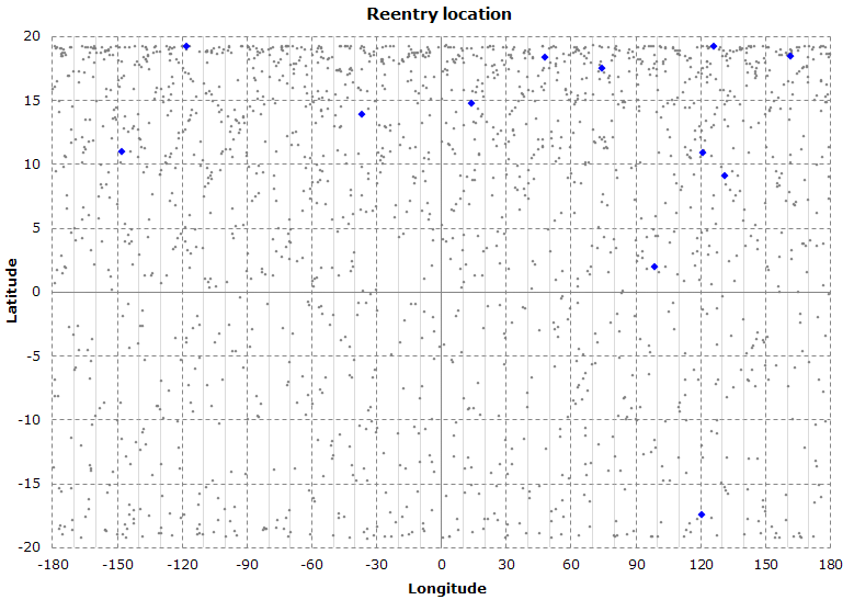
The following map shows the predicted reentry location for each Monte Carlo simulation (the blue dots represent the original, unmodified, TLEs).
If you hover the mouse over a point, a label appears showing the reentry date (TDT) and the TLE epoch.
Here's the same as the above map.
The percentage of the reentry locations in the Northern Hemisphere is now 74.4%.
The graph shows the instantaneous radius vector obtained by propagating the TLE 19059.25918981.
The satellite travels for 274.6 radians in the right ascension and hence the graph shows the last 43.7 orbits.
Simulation date: 2019-02-26
Atmosphere model: NRLMSISE-00, data file: 2019 Feb 26 13:00:02.32
Gravity model: SGG-UGM-1 truncated to degree and order 15
Reentry date: 2019-03-02.8 ± 2.9 days @ 90% confidence level (2019-02-27.9 ÷ 2019-03-05.7)
Here's the result of a Monte Carlo simulation used to calculate the reentry date and the reentry location.
There are no significant differences compared to the last two simulations.
The graph shows the predicted reentry location for each Monte Carlo simulation (the blue dots represent the original, unmodified, TLEs).
The percentage of the reentry locations in the Northern Hemisphere has further increased, now it is 74%.
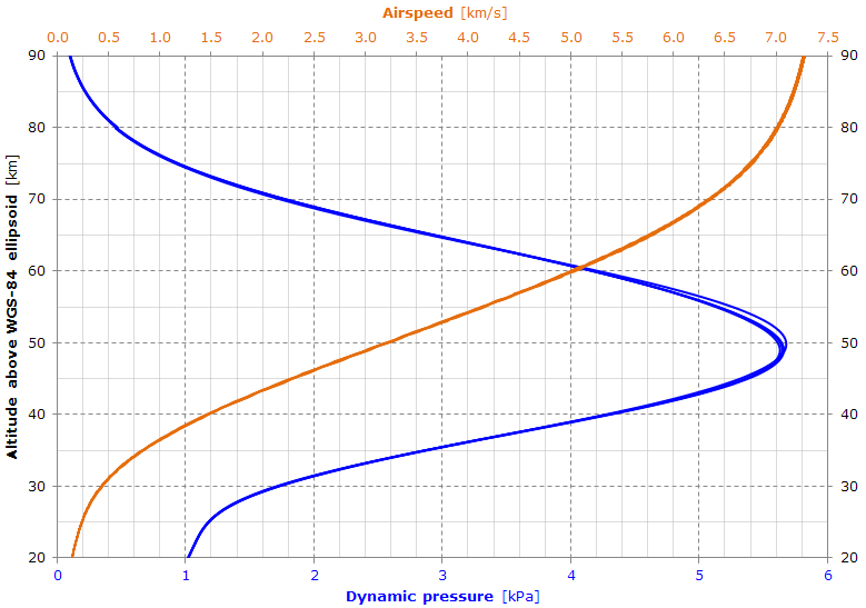
The graph shows a possible reentry profile of the dynamic pressure and satellite airspeed (corotating atmosphere assumed) obtained from the newest 4 TLEs.

Here is shown the approximate stagnation point heat development during reentry.
Simulation date: 2019-02-22
Atmosphere model: NRLMSISE-00, data file: 2019 Feb 22 07:00:02.30
Gravity model: SGG-UGM-1 truncated to degree and order 15
Reentry date: 2019-03-02.6 ± 5.5 days @ 90% confidence level (2019-02-25 ÷ 2019-03-08)
Here's the result of a Monte Carlo simulation used to calculate the reentry date and the reentry location.
There are no significant changes from the previous simulation.
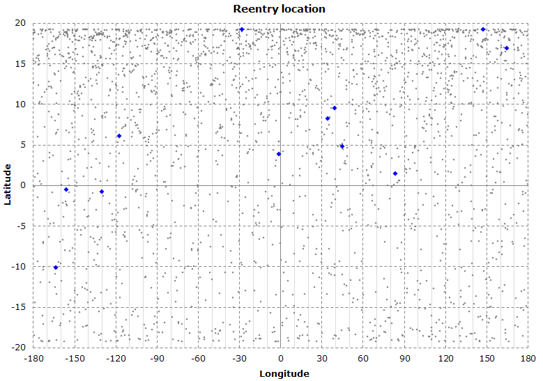
The graph shows the predicted reentry location for each Monte Carlo simulation (the blue dots represent the original, unmodified, TLEs).
Also this simulation shows a more probable reentry in the Northern Hemisphere (about 71.8% of the predicted locations).
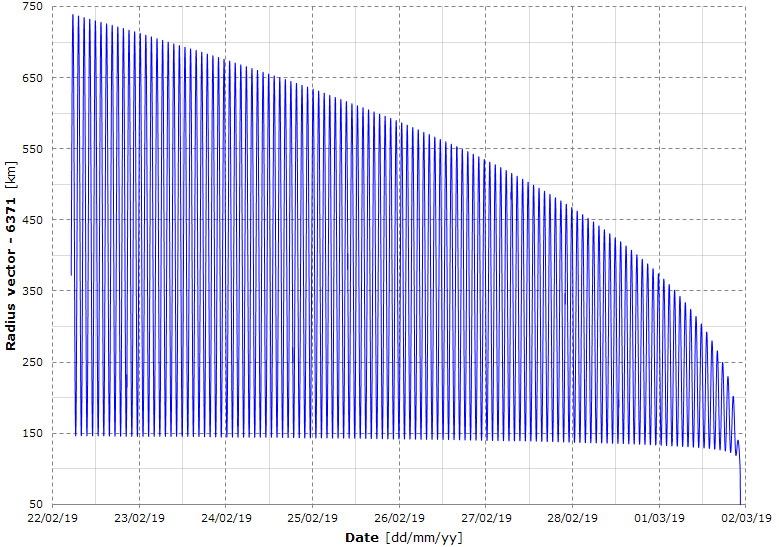
The graph shows the instantaneous radius vector obtained by propagating the TLE 19053.21462918.
The satellite travels for 765.2 radians in the right ascension and hence the graph shows the last 121 orbits.
We see that the perigee radius vector no longer oscillate (see, for example, the simulation 2018-11-21); it is now continuously decaying.
Simulation date: 2019-02-13
Atmosphere model: NRLMSISE-00, data file: 2019 Feb 13 13:00:02.51
Gravity model: SGG-UGM-1 truncated to degree and order 15
Reentry date: 2019-03-02 ± 9 days @ 90% confidence level (2019-02-21 ÷ 2019-03-11)
Here's the result of a Monte Carlo simulation used to calculate the reentry date and the reentry location.
Twelve TLEs have been used, but the graph seems to show only 9 TLEs because some of them overlap (you can count the blue dots shown in the next graph).
The graph shows the predicted reentry location for each Monte Carlo simulation (the blue dots represent the original, unmodified, TLEs).
This simulation starts to show some reentry orbits.
About 71% of the predicted locations lie in the Northern Hemisphere.
Simulation date: 2019-01-25
Atmosphere model: NRLMSISE-00, data file: 2019 Jan 25 13:00:02.24
Gravity model: SGG-UGM-1 truncated to degree and order 15
Reentry date: 2019-03-04 ± 16 days @ 90% confidence level (2019-02-16 ÷ 2019-03-20)
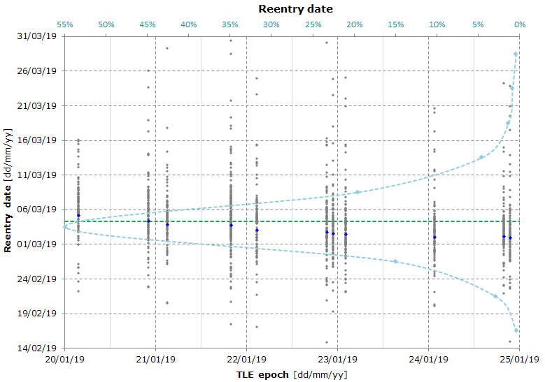
The graph is the result of a Monte Carlo simulation used to calculate the reentry date and the reentry location (the graph of the reentry location is not published as it shows a totally random pattern).
Simulation date: 2019-01-13
Atmosphere model: NRLMSISE-00, data file: 2019 Jan 13 13:00:02.48
Gravity model: SGG-UGM-1 truncated to degree and order 15
Reentry date: 2019-02-23 ± 17 days @ 90% confidence level (2019-02-06 ÷ 2019-03-12)
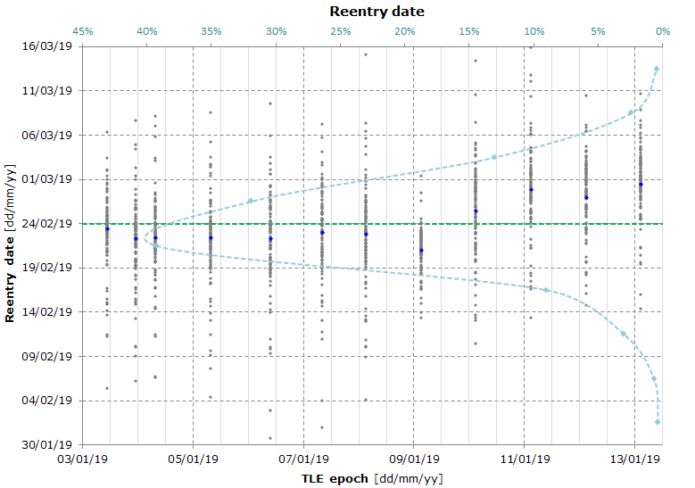
The graph is the result of a Monte Carlo simulation used to calculate the reentry date and the reentry location (the graph of the reentry location is not published as it shows a totally random pattern).
Simulation date: 2018-12-09
Atmosphere model: NRLMSISE-00, data file: 2018 Dec 09 19:00:02.27
Gravity model: SGG-UGM-1 truncated to degree and order 15
Reentry date: 2019-02-20 ± 32 days @ 90% confidence level (2019-01-19 ÷ 2019-03-24)
Starting from this simulation, a much improved model for the TLEs uncertainty is used.
Before this simulation, the TLEs uncertainty was modeled by adding to the satellite radius vector and velocity a normally distributed random offset in the radial, in-track and cross-track directions.
Now the TLEs uncertainty is modeled with a much improved analysis of the IRNSS-1H TLEs (247 TLEs have been used, starting from the TLE 18240). This makes possible to calculate a more reliable confidence interval for the reentry date.
The graph is the result of a Monte Carlo simulation used to calculate the reentry date and the reentry location (the graph of the reentry location is not published as it shows a totally random pattern).
Simulation date: 2018-11-21
Atmosphere model: NRLMSISE-00, data file: 2018 Nov 21 13:00:02.34
Gravity model: SGG-UGM-1 truncated to degree and order 15
Average reentry date: 2019-03-20
The graph is the result of a Monte Carlo simulation (which took 8h 17m CPU time) used to calculate the reentry date and the reentry location.
The graph shows the predicted reentry location for each Monte Carlo simulation (the blue dots represent the original, unmodified, TLEs).
About 65% of the predicted locations lie in the Southern Hemisphere.
Here's the predicted trajectory obtained from the newest 5 TLEs. The plots represent the average, minimum and maximum radius vector scaled to a sphere with a radius of 6371 km (just to show an approximate altitude).
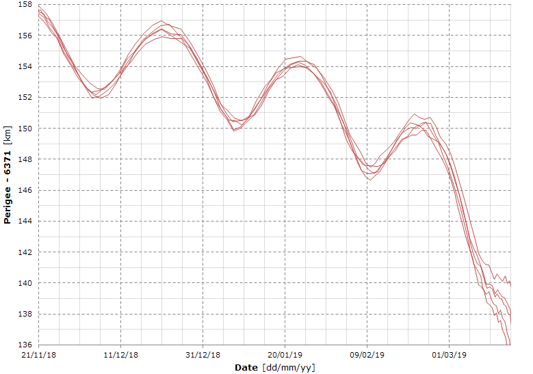
Here's the detailed view of the predicted perigee.
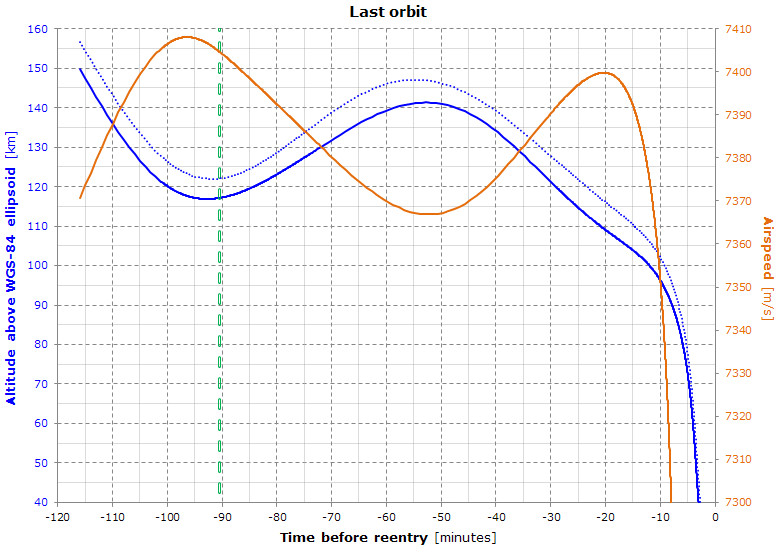
Here's the shape of the predicted last orbit and the corresponding airspeed (corotating atmosphere assumed).
The vertical green line represents the starting time of the last orbit. In this simulation, the last orbit starts about 90 minutes before reentry, at an altitude of about 120 km. The dotted blue plot represents the radius vector minus 6371 km.
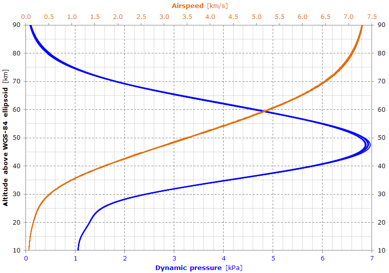
The graph shows a possible reentry profile of the dynamic pressure and satellite airspeed (corotating atmosphere assumed) obtained from the newest 5 TLEs.
If we compare this graph with the
SFERA 2 graph, we see a much higher max-q. The reason is that the SFERA 2 ballistic coefficient is about 40 kg/m
2, while the one of the IRNSS-1H is about 105 kg/m
2.
However, it's totally possible that most of the satellite will disintegrate well above the max-q altitude.
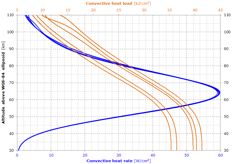
Here is shown the approximate stagnation point heat development during reentry.
Simulation date: 2018-10-15
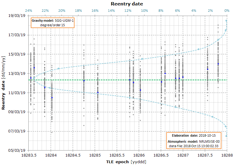
The graph is the result of a Monte Carlo simulation used to calculate the reentry date.
The average reentry date is 2019-03-12. The 95% confidence interval based only on the variance of the reentry dates is ±7.3 days.
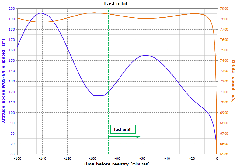
Here's the shape of the predicted last orbit and the corresponding orbital speed.
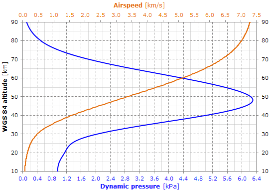
The graph shows a possible reentry profile for the dynamic pressure and the satellite airspeed (corotating atmosphere assumed).
The peak dynamic pressure is relatively small. Just for comparison, for the Tiangong-1 it was about 8.6 kPa.
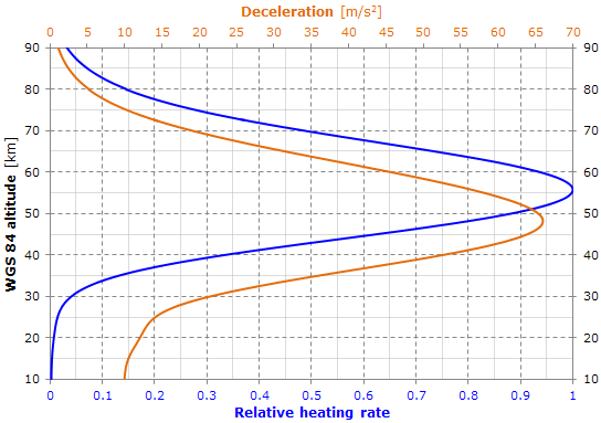
Here's the deceleration of the satellite and the heating rate caused by the atmospheric friction.
The heating rate is proportional to the product of the air density and the cube of the airspeed.
The term "relative" is because the graph shows the value of the heating rate divided by the maximum value of the heating rate.
Simulation date: 2018-09-08
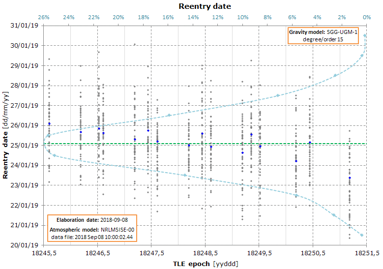
The graph is the result of a Monte Carlo simulation used to calculate the reentry date.
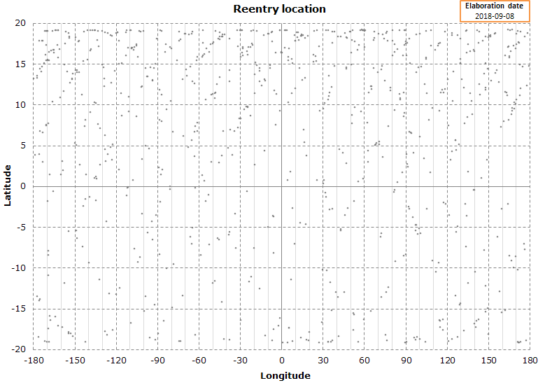
The graph shows the predicted reentry location for each Monte Carlo simulation.
Interestingly enough, this simulation starts to show a clear pattern for the reentry location (the previous graphs were totally random).